![]() May 13
May 13
Kuwait Sugar Consumption with R
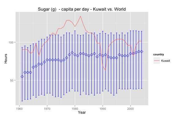
I was doing Facebook’s Udacity Explorartory Data Analysis course and one of the tasks is to use GapMinder.org’s data to visualise data.
So I picked sugar consumption per capita per day; diabetes is a subject that has always been close and interesting to me. The graph above shows Kuwait’s sugar consumption relative to world averages.
Interesting that Kuwait has always been above the median and peaked in the 80’s – maybe that’s why obesity is such a prevalent issue nowadays. In 1990 the drop is, perhaps, due to a lack of data or perhaps due to an exodus of people. Nevertheless it seems that Kuwait has a long way to go in health awareness insofar as sugar consumption is concerned. Sugar consumption is lower today but still above the world median.
Want to reproduce this? Here’s the code – make sure to download the data set first! – :
# Data Cleansing data<-read.csv(file="gapminder.csv",na.strings="NA",row.names=1, header=T, blank.lines.skip=T) data<-(data.frame(t(data))) data<-data.frame(year=c(1961:2004), data) View(data) # Data Pivot library(reshape) data.melt<-melt(data,id='year',variable_name="country") data.melt<-subset(data.melt, value!='NA') data.melt.kuwait<-subset(data.melt, country=='Kuwait') data.melt.other<-subset(data.melt, country!='Kuwait') # Grouping data library('dplyr') year_group <- group_by(data.melt.other, year) wmsub.year_group <- summarise(year_group, mean=mean(value), median=median(value), lowerbound=quantile(value, probs=.25), upperbound=quantile(value, probs=.75)) # Plotting ggplot(data = wmsub.year_group, aes(x = year, y=median))+ geom_errorbar(aes(ymin = lowerbound, ymax = upperbound),colour = 'blue', width = 0.4) + stat_summary(fun.y=median, geom='point', shape=5, size=3, color='blue')+ geom_line(data=data.melt.kuwait, aes(year, value, color=country))+ ggtitle('Sugar (g) - capita per day - Kuwait vs. World')+ xlab('Year') + ylab('Hours') |
![]() May 11
May 11
Install R Package automatically … (if it is not installed)
This is perhaps my favourite helper function in R.
usePackage <- function(p) { if (!is.element(p, installed.packages()[,1])) install.packages(p, dep = TRUE) require(p, character.only = TRUE) } |
Why? Well …
Have you ever tried to run a line of R code that needed a special function from a special library.
The code stops and you think, “Damn … ok I’ll just load the library” – and you do.
But you get an error message because you don’t have the library installed … ya! #FacePalm
After the momentary nuisance you then have to:
- Type in the command to install the package
- Wait for the package to be installed
- Load the library
- Re-run the code
- Eat a cookie
Well that’s why this is my favourite helper function. I just use “usePackage” instead of “library” or “install.packages”. It checks if the library exists on the machine you are working on, if not then the library will be installed, and loaded into the environment of your workspace. Enjoy!
You can even use this as part of your R profile 🙂
![]() May 4
May 4
Tweet Bayes Classification: Excel and R

Foreward

I started reading Data Smart by John Foreman. The book is a great read because of Foreman’s humorous style of writing. What sets this book apart from the other data analysis books I have come across is that it focuses on the techniques rather than the tools – everything is accomplished through the use of a spreadsheet program (e.g. Excel).
So as a personal project to learn more about data analysis and its applications, I will be reproducing exercises in the book both in Excel and R. I will be structured in the blog posts: 0) I will always repeat this paragraph in every post 1) Introducing the Concept and Data Set, 2) Doing the Analysis with Excel, 3) Reproducing the results with R.
If you like the stuff here, please consider buying the book.
Shortcuts
This post is long, so here is a shortcut menu:
Excel
- Step 1: Data Cleaning
- Step 2: Word Counting
- Step 3: Tokenization
- Step 4: Model Building
- Step 5: Using Bayes and the MAP model
R
- Step 1: Data Cleaning
- Step 2: Word Counting
- Step 3: Tokenization
- Step 4: Model Building
- Step 5: Using Bayes and the MAP model
- Entire Code
Tweet Classification
The problem we are going to tackle here is one of classification. We want to know if blocks of texts can be classified into groups based on some model that we build. Specifically we are going to work with a small data set of tweets that have been pre-classified to make a model that will classify new tweets that we have not seen before.
We will be using a Naïve Bayes Classification model. This technique is useful not just for tweets, it can be used for any type of natural language classification: for example e-mail/sms spam filters, loan application risk screening, blog domain classification.
 The case is about Mandrill.com who are monitoring tweets with the tag “Mandrill”. We want to be able to classify tweets automagically into two categories: “relevant” and “irrelevant”.
The problem is that Mandrill is not necessarily a unique word. I searched Twitter for Mandrill and I get 5 tweets that are relevant, and 2 that are not … and the rest do not fit in my screenshot. There are many irrelevant ones beyond that … so do we just get trolled by the rest of the mandrill tweets?
Nope! Lets get started.
Download the vanilla excel files here:
Mandrill – Vanilla
Tweet Classification with Naive Bayes Classifier: Excel
In your Excel file you will have 3 tabs each containing tweets. The first tab contains 150 relevant tweets, the second tab labeled “AboutOther” contains irrelevant tweets, and the last tab has tweets we will use to test the model we are about to develop.
Step 1: Data Cleaning
We will need to do the following for data in the first two tabs. Repeat everything in step 1 for the “AboutMandrilApp” and “AboutOther” tabs.
The first thing we need to do is make everything in non-capital letters. This is done by using the lower() formula. Let us place the formula in cell B2 and drag the formula down to cell B151.
=lower(A2) |
Next we need to swap punctuation with spaces. Specifically we swap these characters with spaces: “. “, “: “, “?”, “!”, “;”, “,”. Note the space after the full-stop and the colon is important. We need to add six columns in each tab use the substitute() function. Place the following 6 in cells C2,D2,E2,F2,G2 and drag them down to row 151:
=SUBSTITUTE(B2,". "," ") =SUBSTITUTE(C2,": "," ") =SUBSTITUTE(D2,"?"," ") =SUBSTITUTE(E2,"!"," ") =SUBSTITUTE(F2,";"," ") =SUBSTITUTE(G2,","," ") |
You can skip this step by downloading the file with this step completed: Mandrill – Step 1
Step 2: Word Counting
Tokenization just means splitting up our sentences (in this case tweets) word by word. Naturally words are split by spaces so we will be using ” ” to split our words. The goal is to have a list of all the words separately in a list. This means we need to figure out how many words we have per tweet to understand how many rows we will need.
We can count the number of words per line by counting the number of spaces in a sentence and adding 1. For example: “The red fox runs fast” has 4 spaces and 5 words. To count spaces we need to subtract the number of characters in a sentence with spaces from the number of characters in the same sentence without spaces. In our example, that would be 21 – 17 which is 4 spaces … and therefore 5 words! This is easily achieved with the following formula copied into column i:
=IF(LEN(TRIM(H2))=0,0,LEN(TRIM(H2))-LEN(SUBSTITUTE(H2," ",""))+1) |
We then see that the maximum number of words is 28 … so we will be safe and take 30 words per sentence. We have 150 tweets, and 30 words per tweet, so we will need 4500 rows for all the words.
Great! We need 2 new tabs now: one called MandrillTokens and the other OtherTokens. Label cell A1 in each of these tabs “Tweet”. Next, copy cell H2 from the MandrillApp tab. Highlight cells A2 to A4501 in the MandrillTokens tab and paste only the values into the cells. This can be accomplished by using the Paste Special option in the Edit menu. You will notice that the tweets will repeat after row 151, this is good since we need to use the same tweet at least 30 times. Repeat this for OtherTokens.
We are now ready to Tokenize! (Wohoo!!)
You can skip this step by downloading the file with this step completed: Mandrill – Step 2
Step 3: Tokenization
Now that we have our tweet set up we need to count words. Since we know words exist between spaces, we need to look for spaces (pretty ironic!). We start by simply placing 0 for cells B2:B151 in MandrillTokens since we start at the very first word – position 0.
We then jump to cell B152 and we can count that the first space starts after 7 letters. To get excel to do this we need to use the find formula to find the space after position 0 (the value in cell B2). Now what if we had a tweet that was empty? We would get an error because there is no space after the first. In that case, we will get an error … so we just want to add 1 to the size of the tweet each time we get an error. This is accomplished with this formula in cell B152:
=IFERROR(FIND(" ",A152,B2+1),LEN(A152)+1) |
You can now safely copy this formula all the way down to cell B4501 giving us all the space positions for all the tweets. Repeat this step for the OtherApps tab.
We can now finally extract each word. We want to get the word between spaces and we now have the position of each space. So in cell C2 we would use the formula:
=IFERROR(MID(A2,B2+1,B152-B2-1),".") |
Which takes the word that starts at letter 1 (Cell B2+1) and ends at letter 7 (Cell B152 – 1 – Cell B2). If there is no word there, we will just place a dot. Copy and paste this formula all the way until cell A4501 and repeat the step for the OtherApps tab.
In column D we want to count the length of each word so place the following formula in D2 and copy it down for the rest of the cells:
=LEN(C2) |
Great, now we’re ready to build our model!
You can skip this step by downloading the file with this step completed: Mandrill – Step 3
Step 4: Model Building
Lets create a pivot table from the information in MandrillTokens in a new tab called MandrillProbability.
Set up your pivot table with “Length” in report filter, “Word” in Row labels, and “Count of Word” in values.
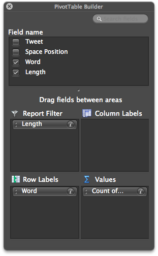
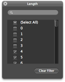
We also want to remove any words that are less than 4 characters long. We do this using the report filter drop-down menu and unchecking 0,1,2, and 3.
Now we need to do what is called additive smoothing: this protects your model against misrepresenting words that rarely appear – e.g. bit.ly urls are unique and so rarely appear. This is a very complicated way of saying “add 1 to everything” … in column C add 1 to all the rows in Column B and then sum them up! Your sheet should now look like this:
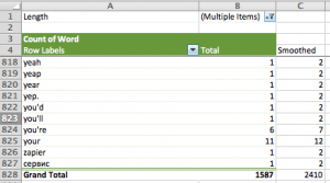
Now we can calculate the probabilities by dividing each cell in column C by the total of column C:
=C5/$C$828 |
The first thing you will notice is that the probabilities are tiny. In larger data sets they will be even tinier and perhaps Excel will not be able to handle it. So we take the natural log of the numbers using the LN() function in column D:
=LN(D5) |
Repeat all these steps for the AboutOther tab and create an Other Probability tab.
You can skip this step by downloading the file with this step completed: Mandrill – Step 4
That’s it believe it or not! You have a model.
Step 5: Using Bayes and the MAP model
So we are at a stage where we have probabilities for words in the “relevant” tweets and “irrelevant” tweets. Now what? We will now use the Maximum A Posteriori (MAP) rule that basically says, given a word if the probability of it being classified as “relevant” is higher than “irrelevant, then it’s “relevant”.
Lets demonstrate with the “TestTweets” tab. First you need to process the tweets again like we did before:
=SUBSTITUTE(B2,". "," ") =SUBSTITUTE(C2,": "," ") =SUBSTITUTE(D2,"?"," ") =SUBSTITUTE(E2,"!"," ") =SUBSTITUTE(F2,";"," ") =SUBSTITUTE(G2,","," ") |
Then create a tab called “Predictions”. In cell A1 input the label “Number” and in A2 to A21 put in the numbers 1 through 20. Label cell B2 “Prediction”. Copy and paste the values from the “TestTweets” column into C2.
Now we need to tokenize the tweets in column C. It is a lot easier this time around. All you have to do is highlight cells C2 to C21 and select “Text to Column” from the “Data” menu. You will see a pop-up screen, click next and then select “Spaces”:
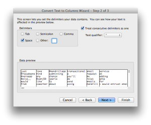
Click next and in the final screen input $D$2 as the destination cell. That’s it! All tokenized and ready for predictions … which is going to get messy 🙂
What we need to do is take each token and look up the probabilities in the “Mandrill Probability” tab and in the “Other Probability” tab. Start in cell D25 and use VLookUp() as follows:
=VLOOKUP(D2,'Mandrill Probability'!$A$5:$E$827,5,FALSE) |
Which says look up the value of D2 in the range of cells in the Mandrill Probability tab, and if you find the token, return the value in column 5 of the Mandrill Probability tab – which is the probability.
The problem here is that if you do not find the word you will have a case of a “rare word” … which we need to replace with the natural log of 1 / total smoothed tokens. So our formula will now use an if() statement and the NA() function which returns 1 or 0 if the value is found or not found respectively. We also want to throw away tokens that are shorter than 4 letters long. So we need yet another if() statement … and here is the monstrosity:
=IF(LEN(D2)<=3,0,IF(ISNA(VLOOKUP(D2,'Mandrill Probability'!$A$5:$E$827,5,FALSE)), LN(1/'Mandrill Probability'!$C$828),VLOOKUP(D2,'Mandrill Probability'!$A$5:$E$827,5,FALSE))) |
Now you can drag this down to D44 through to AI44.
Repeat this in D48 to AI for the ‘Other Probability’:
=IF(LEN(D2)<=3,0,IF(ISNA(VLOOKUP(D2,'Other Probability'!$A$5:$E$810,5,FALSE)), LN(1/'Other Probability'!$C$811),VLOOKUP(D2,'Other Probability'!$A$5:$E$810,5,FALSE))) |
Almost there, now we need to sum up each row. In cell B25 input:
=SUM(D25:AI25) |
Copy this down to B67. Now we need to compare if the top set of numbers is greater than the bottom set of numbers in our predictions. In cell B2, input the comparison:
=IF(B25>B48,"APP","OTHER") |
Drag this down to B20 to get the predictions!
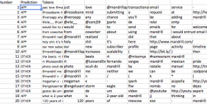
Of the 20 predicted, the model only makes a mistake on 1. That’s a pretty good margin of error.
All you need to do is repeat the steps for new tweets in the last tab. The model will deteriorate over time and therefore it is important to continuously update the model for better prediction.
You can skip this step by downloading the file with this step completed: Mandrill – Step 5
Tweet Classification with Naive Bayes Classifier: R
Step 1: Data Cleaning
We start off with our vanilla data set separated into 3 different files:
Download those files into your working directory and fire up R.
The first thing we need to do is load up the libraries we will be using and read our data. We also add the appropriate columns for “App” and “Other”:
# Libraries library(tm) # Collect data tweets.mandrill<-read.csv('Mandrill.csv',header=T) tweets.other<-read.csv('Other.csv',header=T) tweets.test<-read.csv('Test.csv',header=T) # Add "App" to mandrill tweets, and "Other" to others. tweets.mandrill["class"]<-rep("App",nrow(tweets.mandrill)) tweets.other["class"]<-rep("Other",nrow(tweets.mandrill)) |
We then need a helper function to replace all the stuff we do not want in the tweets. To do this we use a function called gsub() within our helper function.
# Helper Function replacePunctuation <- function(x) { x <- tolower(x) x <- gsub("[.]+[ ]"," ",x) x <- gsub("[:]+[ ]"," ",x) x <- gsub("[?]"," ",x) x <- gsub("[!]"," ",x) x <- gsub("[;]"," ",x) x <- gsub("[,]"," ",x) x } |
Let us do the text transformations on our tweets now:
# Do our punctuation stuff tweets.mandrill$Tweet <- replacePunctuation(tweets.mandrill$Tweet) tweets.other$Tweet <- replacePunctuation(tweets.other$Tweet) tweets.test$Tweet <- replacePunctuation(tweets.test$Tweet) |
Step 2: Word Counting
We do not need to count words for the R version. Pat yourself on the back for making a smart decision … not too much though this will get messy soon I promise 🙂

Step 3: Tokenization
We are going to use the ‘tm’ library to tokenize our training and test data. First we will create a Corpus – which is just a funky word for a set of text stuff … in this case tweets!
# Create corpus tweets.mandrill.corpus <- Corpus(VectorSource(as.vector(tweets.mandrill$Tweet))) tweets.other.corpus <- Corpus(VectorSource(as.vector(tweets.other$Tweet))) tweets.test.corpus <- Corpus(VectorSource(as.vector(tweets.test$Tweet))) |
Great! Now we want to get a term document matrix – another fancy phrase for a table that shows how many times each word was mentioned in each document.
# Create term document matrix tweets.mandrill.matrix <- t(TermDocumentMatrix(tweets.mandrill.corpus,control = list(wordLengths=c(4,Inf)))); tweets.other.matrix <- t(TermDocumentMatrix(tweets.other.corpus,control = list(wordLengths=c(4,Inf)))); tweets.test.matrix <- t(TermDocumentMatrix(tweets.test.corpus,control = list(wordLengths=c(4,Inf)))); |
This is what the term document matrix looks like:
Terms Docs which whom wisest with wordpress words 10 0 0 0 2 0 0 11 0 0 0 0 0 0 12 0 0 0 0 0 0 13 0 0 0 0 0 0 14 0 0 0 1 0 0 15 0 0 0 0 0 0 |
Great! That’s just what we need; we can count words in documents and totals later!
We can move on to building our model now.
Step 4: Model Building
We want to create the probabilities table.
- We start by counting the number of times each word has been used
- We then need to do the “additive smoothing” step
- We then take then calculate the probabilities using the smoothed frequencies
- Lastly we need to take the natural log of the probabilities
To save us time, we will write a little helper function that will do this for any document matrix we might have.
probabilityMatrix <-function(docMatrix) { # Sum up the term frequencies termSums<-cbind(colnames(as.matrix(docMatrix)),as.numeric(colSums(as.matrix(docMatrix)))) # Add one termSums<-cbind(termSums,as.numeric(termSums[,2])+1) # Calculate the probabilties termSums<-cbind(termSums,(as.numeric(termSums[,3])/sum(as.numeric(termSums[,3])))) # Calculate the natural log of the probabilities termSums<-cbind(termSums,log(as.numeric(termSums[,4]))) # Add pretty names to the columns colnames(termSums)<-c("term","count","additive","probability","lnProbability") termSums } |
Great, now we can just use that for our training sets “App” and “Other”.
tweets.mandrill.pMatrix<-probabilityMatrix(tweets.mandrill.matrix) tweets.other.pMatrix<-probabilityMatrix(tweets.other.matrix) |
We can output these to files and compare them to the Excel file:
write.csv(file="mandrillProbMatrix.csv",tweets.mandrill.pMatrix) write.csv(file="otherProbMatrix.csv",tweets.mandrill.pMatrix) |
Step 5: Using Bayes and the MAP model
We now want to use the MAP model to compare each of the test tweets with the two probability matrices.
We will write another function to help us out here. We start thinking about what we want to do with each tweet:
- Get each test tweets characters and look for them in a probability matrix
- We want to know how many words were not found.
- We want to sum up the probabilities of the found words
- For the words we do not find, we want to add ln(1/sum of the smoothed words) each time
- Sum up the probabilities from the last 2 steps
Lets go:
getProbability <- function(testChars,probabilityMatrix) { charactersFound<-probabilityMatrix[probabilityMatrix[,1] %in% testChars,"term"] # Count how many words were not found in the mandrill matrix charactersNotFound<-length(testChars)-length(charactersFound) # Add the normalized probabilities for the words founds together charactersFoundSum<-sum(as.numeric(probabilityMatrix[probabilityMatrix[,1] %in% testChars,"lnProbability"])) # We use ln(1/total smoothed words) for words not found charactersNotFoundSum<-charactersNotFound*log(1/sum(as.numeric(probabilityMatrix[,"additive"]))) #This is our probability prob<-charactersFoundSum+charactersNotFoundSum prob } |
Now we can use this function for every tweet we have with a for loop. Lets see how this is done:
# Get the matrix tweets.test.matrix<-as.matrix(tweets.test.matrix) # A holder for classification classified<-NULL for(documentNumber in 1:nrow(tweets.test.matrix)) { # Extract the test words tweets.test.chars<-names(tweets.test.matrix[documentNumber,tweets.test.matrix[documentNumber,] %in% 1]) # Get the probabilities mandrillProbability <- getProbability(tweets.test.chars,tweets.mandrill.pMatrix) otherProbability <- getProbability(tweets.test.chars,tweets.other.pMatrix) # Add it to the classification list classified<-c(classified,ifelse(mandrillProbability>otherProbability,"App","Other")) } |
Brilliant we can take a look at our classification alongside our tweets:
View(cbind(classified,tweets.test$Tweet)) |
Very much like our Excel model, we are off by 1/20.
Entire Code
library(tm) # Collect data tweets.mandrill<-read.csv('Mandrill.csv',header=T) tweets.other<-read.csv('Other.csv',header=T) tweets.test<-read.csv('Test.csv',header=T) tweets.mandrill["class"]<-rep("App",nrow(tweets.mandrill)) tweets.other["class"]<-rep("Other",nrow(tweets.mandrill)) # Helper Function replacePunctuation <- function(x) { x <- tolower(x) x <- gsub("[.]+[ ]"," ",x) x <- gsub("[:]+[ ]"," ",x) x <- gsub("[?]"," ",x) x <- gsub("[!]"," ",x) x <- gsub("[;]"," ",x) x <- gsub("[,]"," ",x) x } # Do our punctuation stuff tweets.mandrill$Tweet <- replacePunctuation(tweets.mandrill$Tweet) tweets.other$Tweet <- replacePunctuation(tweets.other$Tweet) tweets.test$Tweet <- replacePunctuation(tweets.test$Tweet) # Create corpus tweets.mandrill.corpus <- Corpus(VectorSource(as.vector(tweets.mandrill$Tweet))) tweets.other.corpus <- Corpus(VectorSource(as.vector(tweets.other$Tweet))) tweets.test.corpus <- Corpus(VectorSource(as.vector(tweets.test$Tweet))) # Create term document matrix tweets.mandrill.matrix <- t(TermDocumentMatrix(tweets.mandrill.corpus,control = list(wordLengths=c(4,Inf)))); tweets.other.matrix <- t(TermDocumentMatrix(tweets.other.corpus,control = list(wordLengths=c(4,Inf)))); tweets.test.matrix <- t(TermDocumentMatrix(tweets.test.corpus,control = list(wordLengths=c(4,Inf)))); # Probability Matrix probabilityMatrix <-function(docMatrix) { # Sum up the term frequencies termSums<-cbind(colnames(as.matrix(docMatrix)),as.numeric(colSums(as.matrix(docMatrix)))) # Add one termSums<-cbind(termSums,as.numeric(termSums[,2])+1) # Calculate the probabilties termSums<-cbind(termSums,(as.numeric(termSums[,3])/sum(as.numeric(termSums[,3])))) # Calculate the natural log of the probabilities termSums<-cbind(termSums,log(as.numeric(termSums[,4]))) # Add pretty names to the columns colnames(termSums)<-c("term","count","additive","probability","lnProbability") termSums } tweets.mandrill.pMatrix<-probabilityMatrix(tweets.mandrill.matrix) tweets.other.pMatrix<-probabilityMatrix(tweets.other.matrix) #Predict # Get the test matrix # Get words in the first document getProbability <- function(testChars,probabilityMatrix) { charactersFound<-probabilityMatrix[probabilityMatrix[,1] %in% testChars,"term"] # Count how many words were not found in the mandrill matrix charactersNotFound<-length(testChars)-length(charactersFound) # Add the normalized probabilities for the words founds together charactersFoundSum<-sum(as.numeric(probabilityMatrix[probabilityMatrix[,1] %in% testChars,"lnProbability"])) # We use ln(1/total smoothed words) for words not found charactersNotFoundSum<-charactersNotFound*log(1/sum(as.numeric(probabilityMatrix[,"additive"]))) #This is our probability prob<-charactersFoundSum+charactersNotFoundSum prob } # Get the matrix tweets.test.matrix<-as.matrix(tweets.test.matrix) # A holder for classification classified<-NULL for(documentNumber in 1:nrow(tweets.test.matrix)) { # Extract the test words tweets.test.chars<-names(tweets.test.matrix[documentNumber,tweets.test.matrix[documentNumber,] %in% 1]) # Get the probabilities mandrillProbability <- getProbability(tweets.test.chars,tweets.mandrill.pMatrix) otherProbability <- getProbability(tweets.test.chars,tweets.other.pMatrix) # Add it to the classification list classified<-c(classified,ifelse(mandrillProbability>otherProbability,"App","Other")) } View(cbind(classified,tweets.test$Tweet)) |


Chatter