![]() Mar 19
Mar 19

Market Basket Analysis with R
Association Rules
There are many ways to see the similarities between items. These are techniques that fall under the general umbrella of association. The outcome of this type of technique, in simple terms, is a set of rules that can be understood as “if this, then that”.
Applications
So what kind of items are we talking about?
There are many applications of association:
- Product recommendation – like Amazon’s “customers who bought that, also bought this”
- Music recommendations – like Last FM’s artist recommendations
- Medical diagnosis – like with diabetes really cool stuff
- Content optimisation – like in magazine websites or blogs
In this post we will focus on the retail application – it is simple, intuitive, and the dataset comes packaged with R making it repeatable.
The Groceries Dataset
Imagine 10000 receipts sitting on your table. Each receipt represents a transaction with items that were purchased. The receipt is a representation of stuff that went into a customer’s basket – and therefore ‘Market Basket Analysis’.
That is exactly what the Groceries Data Set contains: a collection of receipts with each line representing 1 receipt and the items purchased. Each line is called a transaction and each column in a row represents an item. You can download the Groceries data set to take a look at it, but this is not a necessary step.
A little bit of Math
We already discussed the concept of Items and Item Sets.
We can represent our items as an item set as follows:
Therefore a transaction is represented as follows:
This gives us our rules which are represented as follows:
Which can be read as “if a user buys an item in the item set on the left hand side, then the user will likely buy the item on the right hand side too”. A more human readable example is:
If a customer buys coffee and sugar, then they are also likely to buy milk.
With this we can understand three important ratios; the support, confidence and lift. We describe the significance of these in the following bullet points, but if you are interested in a formal mathematical definition you can find it on wikipedia.
- Support: The fraction of which our item set occurs in our dataset.
- Confidence: probability that a rule is correct for a new transaction with items on the left.
- Lift: The ratio by which by the confidence of a rule exceeds the expected confidence.
Note: if the lift is 1 it indicates that the items on the left and right are independent. - We set the minimum support to 0.001
- We set the minimum confidence of 0.8
- We then show the top 5 rules
- The number of rules generated: 410
- The distribution of rules by length: Most rules are 4 items long
- The summary of quality measures: interesting to see ranges of support, lift, and confidence.
- The information on the data mined: total data mined, and minimum parameters.
- What are customers likely to buy before buying whole milk
- What are customers likely to buy if they purchase whole milk?
- We set the confidence to 0.15 since we get no rules with 0.8
- We set a minimum length of 2 to avoid empty left hand side items
- Snowplow Market Basket Analysis
- Discovering Knowledge in Data: An Introduction to Data Mining
- RDatamining.com
Apriori Recommendation with R
So lets get started by loading up our libraries and data set.
# Load the libraries library(arules) library(arulesViz) library(datasets) # Load the data set data(Groceries) |
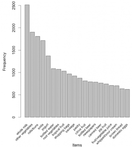
Lets explore the data before we make any rules:
# Create an item frequency plot for the top 20 items itemFrequencyPlot(Groceries,topN=20,type="absolute") |
We are now ready to mine some rules!
You will always have to pass the minimum required support and confidence.
# Get the rules rules <- apriori(Groceries, parameter = list(supp = 0.001, conf = 0.8)) # Show the top 5 rules, but only 2 digits options(digits=2) inspect(rules[1:5]) |
The output we see should look something like this
lhs rhs support confidence lift 1 {liquor,red/blush wine} => {bottled beer} 0.0019 0.90 11.2 2 {curd,cereals} => {whole milk} 0.0010 0.91 3.6 3 {yogurt,cereals} => {whole milk} 0.0017 0.81 3.2 4 {butter,jam} => {whole milk} 0.0010 0.83 3.3 5 {soups,bottled beer} => {whole milk} 0.0011 0.92 3.6 |
This reads easily, for example: if someone buys yogurt and cereals, they are 81% likely to buy whole milk too.
We can get summary info. about the rules that give us some interesting information such as:
set of 410 rules rule length distribution (lhs + rhs): sizes 3 4 5 6 29 229 140 12 summary of quality measures: support conf. lift Min. :0.00102 Min. :0.80 Min. : 3.1 1st Qu.:0.00102 1st Qu.:0.83 1st Qu.: 3.3 Median :0.00122 Median :0.85 Median : 3.6 Mean :0.00125 Mean :0.87 Mean : 4.0 3rd Qu.:0.00132 3rd Qu.:0.91 3rd Qu.: 4.3 Max. :0.00315 Max. :1.00 Max. :11.2 mining info: data n support confidence Groceries 9835 0.001 0.8 |
Sorting stuff out
The first issue we see here is that the rules are not sorted. Often we will want the most relevant rules first. Lets say we wanted to have the most likely rules. We can easily sort by confidence by executing the following code.
rules<-sort(rules, by="confidence", decreasing=TRUE) |
Now our top 5 output will be sorted by confidence and therefore the most relevant rules appear.
lhs rhs support conf. lift 1 {rice,sugar} => {whole milk} 0.0012 1 3.9 2 {canned fish,hygiene articles} => {whole milk} 0.0011 1 3.9 3 {root vegetables,butter,rice} => {whole milk} 0.0010 1 3.9 4 {root vegetables,whipped/sour cream,flour} => {whole milk} 0.0017 1 3.9 5 {butter,soft cheese,domestic eggs} => {whole milk} 0.0010 1 3.9 |
Rule 4 is perhaps excessively long. Lets say you wanted more concise rules. That is also easy to do by adding a “maxlen” parameter to your apriori function:
rules <- apriori(Groceries, parameter = list(supp = 0.001, conf = 0.8,maxlen=3)) |
Redundancies
Sometimes, rules will repeat. Redundancy indicates that one item might be a given. As an analyst you can elect to drop the item from the dataset. Alternatively, you can remove redundant rules generated.
We can eliminate these repeated rules using the follow snippet of code:
subset.matrix <- is.subset(rules, rules) subset.matrix[lower.tri(subset.matrix, diag=T)] <- NA redundant <- colSums(subset.matrix, na.rm=T) >= 1 rules.pruned <- rules[!redundant] rules<-rules.pruned |
Targeting Items
Now that we know how to generate rules, limit the output, lets say we wanted to target items to generate rules. There are two types of targets we might be interested in that are illustrated with an example of “whole milk”:
This essentially means we want to set either the Left Hand Side and Right Hand Side. This is not difficult to do with R!
Answering the first question we adjust our apriori() function as follows:
rules<-apriori(data=Groceries, parameter=list(supp=0.001,conf = 0.08), appearance = list(default="lhs",rhs="whole milk"), control = list(verbose=F)) rules<-sort(rules, decreasing=TRUE,by="confidence") inspect(rules[1:5]) |
The output will look like this:
lhs rhs supp. conf. lift 1 {rice,sugar} => {whole milk} 0.0012 1 3.9 2 {canned fish,hygiene articles} => {whole milk} 0.0011 1 3.9 3 {root vegetables,butter,rice} => {whole milk} 0.0010 1 3.9 4 {root vegetables,whipped/sour cream,flour} => {whole milk} 0.0017 1 3.9 5 {butter,soft cheese, domestic eggs} => {whole milk} 0.0010 1 3.9 |
Likewise, we can set the left hand side to be “whole milk” and find its antecedents.
Note the following:
rules<-apriori(data=Groceries, parameter=list(supp=0.001,conf = 0.15,minlen=2), appearance = list(default="rhs",lhs="whole milk"), control = list(verbose=F)) rules<-sort(rules, decreasing=TRUE,by="confidence") inspect(rules[1:5]) |
Now our output looks like this:
lhs rhs support confidence lift 1 {whole milk} => {other vegetables} 0.075 0.29 1.5 2 {whole milk} => {rolls/buns} 0.057 0.22 1.2 3 {whole milk} => {yogurt} 0.056 0.22 1.6 4 {whole milk} => {root vegetables} 0.049 0.19 1.8 5 {whole milk} => {tropical fruit} 0.042 0.17 1.6 6 {whole milk} => {soda} 0.040 0.16 0.9 |
Visualization
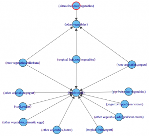
The last step is visualization. Lets say you wanted to map out the rules in a graph. We can do that with another library called “arulesViz”.
library(arulesViz) plot(rules,method="graph",interactive=TRUE,shading=NA) |
You will get a nice graph that you can move around to look like this:
References
Resources
![]() Posted by Salem
Posted by Salem
![]() Feb 25
Feb 25
The Cookie Thief by Valerie Cox

The Cookie Thief
A woman was waiting at an airport one night,
With several long hours before her flight.
She hunted for a book in the airport shops.
Bought a bag of cookies and found a place to drop.
She was engrossed in her book but happened to see,
That the man sitting beside her, as bold as could be.
Grabbed a cookie or two from the bag in between,
Which she tried to ignore to avoid a scene.
So she munched the cookies and watched the clock,
As the gutsy cookie thief diminished her stock.
She was getting more irritated as the minutes ticked by,
Thinking, “If I wasn’t so nice, I would blacken his eye.â€
With each cookie she took, he took one too,
When only one was left, she wondered what he would do.
With a smile on his face, and a nervous laugh,
He took the last cookie and broke it in half.
He offered her half, as he ate the other,
She snatched it from him and thought… oooh, brother.
This guy has some nerve and he’s also rude,
Why he didn’t even show any gratitude!
She had never known when she had been so galled,
And sighed with relief when her flight was called.
She gathered her belongings and headed to the gate,
Refusing to look back at the thieving ingrate.
She boarded the plane, and sank in her seat,
Then she sought her book, which was almost complete.
As she reached in her baggage, she gasped with surprise,
There was her bag of cookies, in front of her eyes.
If mine are here, she moaned in despair,
The others were his, and he tried to share.
Too late to apologize, she realized with grief,
That she was the rude one, the ingrate, the thief.
![]() Feb 24
Feb 24
Harvesting Tweets with R
Problem Definition

If you are a regular Twitter user, you’ll find yourself wanting to collect all your tweets for whatever obscure reason. I was looking to do some sort of sentiment analysis on a large dataset – it made sense to go to Twitter … but you can only get 1500 tweets at a time with Twitter’s API.
After looking around forums I couldn’t find a reasonable solution. So one way to tackle this is to build up a database over time – just store the tweets you want locally. Since I was going to use this with R, I wanted to collect data with R.
To do this, we can use the twitteR package to communicate with Twitter and save our data.
Once you have the script in place, you can run a cron job to execute the script every day, week, hour or whatever you see fit.
Connecting to Twitter
We will be using 3 libraries in our R Script. Lets load them into our environment:
library(twitteR) library(RCurl) library(ROAuth) |
We will need to set up an SSL certificate (especially if you are on Windows). We do this using the following line of code:
options(RCurlOptions = list(cainfo = system.file("CurlSSL", "cacert.pem", package = "RCurl"))) |
Lets set up our API variables to connect to twitter.
reqURL <- "https://api.twitter.com/oauth/request_token" accessURL <- "https://api.twitter.com/oauth/access_token" authURL <- "http://api.twitter.com/oauth/authorize" |
You will need to get a api key and api secret from Twitter’s developer site https://apps.twitter.com/app/new – make sure you give read, write, and direct message permissions to your newly created application.
apiKey <- "YOUR-KEY" apiSecret <- "YOUR-SECRET" |
Lets put everything together and try an authorize our application.
twitCred <- OAuthFactory$new( consumerKey=apiKey, consumerSecret=apiSecret, requestURL=reqURL, accessURL=accessURL, authURL=authURL) |
Now lets connect by doing a handshake …
twitCred$handshake() |
You will get a message to follow a link and get a confirmation code to input into your R console. The message will look like this:
To enable the connection, please direct your web browser to: http://api.twitter.com/oauth/authorize?oauth_token=4Ybnjkljkljlst5cvO5t3nqd8bhhGqTL3nQ When complete, record the PIN given to you and provide it here:
Now we can save our credentials for next time!
registerTwitterOAuth(twitCred) save(list="twitCred", file="credentials") |
Harvesting Tweets
Now that we are connected we can put in our queries:
- We will use a comma separated string of key words we want to track.
- Once we define our string of key words, we split the string and make a list.
- We will also need a variable to hold our tweets.
I chose key words related to Kuwait.
query <- "kuwaiti,kuwait,#kuwait,#q8" query <- unlist(strsplit(query,",")) tweets = list() |
Now we are ready to ask Twitter for tweets on our key words. What we do in the following block of code is loop through our string of key words; in this case we loop 4 times for our 4 key words.
We use twitteR’s function searchTwitter() which takes the query as a parameter. We also supply additional parameters: n – the number of tweets, geocode – a latitude, longitude and radius (in our example we use within an 80 mile radius of Kuwait City).
for(i in 1:length(query)){ result<-searchTwitter(query[i],n=1500,geocode='29.3454657,47.9969453,80mi') tweets <- c(tweets,result) tweets <- unique(tweets) } |
That’s it, we have our data. All that needs to be done now is save it.
R does not allow you to append data to CSV files, so what we will do is:
- Check if there is a file called tweets.csv and read the data in there
- Merge the data already in the CSV file with our new data
- Remove any duplicates in the data
- Save the file as tweets.csv again
# Create a placeholder for the file file<-NULL # Check if tweets.csv exists if (file.exists("tweets.csv")){file<- read.csv("tweets.csv")} # Merge the data in the file with our new tweets df <- do.call("rbind", lapply(tweets, as.data.frame)) df<-rbind(df,file) # Remove duplicates df <- df[!duplicated(df[c("id")]),] # Save write.csv(df,file="tweets.csv",row.names=FALSE) |
Code
For your convenience, the code in one block:
# Load libraries library(twitteR) library(RCurl) library(ROAuth) # SSL Certificate options(RCurlOptions = list(cainfo = system.file("CurlSSL", "cacert.pem", package = "RCurl"))) # API URLs reqURL <- "https://api.twitter.com/oauth/request_token" accessURL <- "https://api.twitter.com/oauth/access_token" authURL <- "http://api.twitter.com/oauth/authorize" # API Keys from https://apps.twitter.com/app/new apiKey <- "YOUR-KEY" apiSecret <- "YOUR-SECRET" # Connect to Twitter to get credentials twitCred <- OAuthFactory$new( consumerKey=apiKey, consumerSecret=apiSecret, requestURL=reqURL, accessURL=accessURL, authURL=authURL) # Twitter Handshake - you will need to get the PIN after this twitCred$handshake() # Optionally save credentials for later registerTwitterOAuth(twitCred) save(list="twitCred", file="credentials") # Set up the query query <- "kuwaiti,kuwait,#kuwait,#q8" query <- unlist(strsplit(query,",")) tweets = list() # Loop through the keywords and store results for(i in 1:length(query)){ result<-searchTwitter(query[i],n=1500,geocode='29.3454657,47.9969453,80mi') tweets <- c(tweets,result) tweets <- unique(tweets) } # Create a placeholder for the file file<-NULL # Check if tweets.csv exists if (file.exists("tweets.csv")){file<- read.csv("tweets.csv")} # Merge the data in the file with our new tweets df <- do.call("rbind", lapply(tweets, as.data.frame)) df<-rbind(df,file) # Remove duplicates df <- df[!duplicated(df[c("id")]),] # Save write.csv(df,file="tweets.csv",row.names=FALSE) # Done! |
![]() Posted by Salem
Posted by Salem


Chatter